Remote Sensing Lab 6: Geometric Correction

Part 1: Image to Map Rectification:

Step 1: Bring the image Chicago_drg.img into Erdas 2013.

Step 2: Next, open a second viewer in Erdas 2013 and bring in Chicago_2000.img. Fit both images to frame.

Step 3: Making sure that the viewer with Chicago_2000.img is active, activate the Multispectral tools and click on Control Points. This will open the Set Geometric Model dialogue box.

a)      Under Select Geometric Model, choose Polynomial followed by OK.

b)      A GCP Tool Reference Setup dialogue box will now open in addition to the Multipoint Geometric Correction dialogue box. Leave the default value in the GCP Tool Reference box as they are, i.e. Image Layer (New Viewer) and click OK to close it out.

c)      Navigate to the appropriate folder and select Chicago_drg.img to add as the reference image.

d)      Click OK on the reference Map Information dialogue box.

e)      A new dialogue box called Polynomial Model Properties will now open. A first order polynomial equation will be used to develop the model that will be used to rectify Chicago_2000.img. Accept the default values of this box and click Close to close it out.

f)       Maximize the Multipoint Correction Window. The window should be contain 6 panes, three for each image, and should look similar to figure 1.

g)      Delete the default GCPs that are at the bottom of the screen. Use Shift to select the values and delete them by click on them with the right mouse button.

h)      Fit the largest Chicago_2000.img to window (right mouse button); do the same for Chicago_drg.img.

i)        Click the Create GCP tool in the Multipoint Geometric Correction interface. It looks like a large cross-hair. This action will turn the cursor into a cross-hair on the screen as well.

j)        Add the first GCP to the Chicago_2000.img and do the same to the reference image on the right-hand side of the Multipoint Correction interface.

k)      Repeat the same process until GCPs 1-4 are roughly in the same areas as those in figure 1. Notice that the GCPs are spread across the images, this helps to ensure a better rectification than if all GCPs were located in close proximity to one another. At this point, having the GCP exactly corresponding to one another is not detrimental, but it will be later. Notice that the bottom of the Multipoint Correction interface now reads ‘Model Solution is Current.’ This is because there are enough GCPs to run a 1^st order polynomial model.

l)        Next, the Root Mean Square (RMS) error will need to be adjusted. Total RMS is indicated in the bottom right-hand corner of the Multipoint Correction interface. Under the heading: Control Point Error Total. In order to run a good model, total Control Point Error should be less than 0.5.

m)   Adjust the RMS by zooming in on a GCP and adjusting it until the RMS is at the desired value. This part may be very tedious, but it generally helps to get the RMS close (e.g. less than 15) and then zoom in on a particular GCP and adjust until the X and Y values in the Control Point Error section of the interface each read as close to zero as possible.

Figure 1

  A)

 

B)

 

Figure 1a shows how the Multipoint Correction interface should appear and the approximate locations of the GCPs. Figure 1b shows the Total Control Point Error which should be less than 0.5.

n)      Once the RMS value is at the appropriate level, click Display Resample Image dialogue button at the top of the Multipoint Correction interface.

o)      Name the output file Chicago_2000gcr.img.

p)      Leave all parameters at their default values and click OK to run the model.

q)      Click Dismiss when the model is finished running. DO NOT SAVE CURRENT GEOMETRIC MODEL.

Q1 What function(s) did the image Chicago_drg.img performed in the geometric correction process? [Hint: you should name and describe the interpolation that this image aided in the process of geometrically correcting the Chicago_2000.img image].

Chicago_drg.img was for the spatial interpolation portion of the geometric correction process. In this case, a first order (linear) polynomial function was used in order fit the data derived from GCPs placed on each image in the Multipoint Correction interface in Erdas. If the image were more distorted a higher order polynomial function would have been more appropriate to use; however, doing this would also require a larger minimum of GCPs to be collected as well.

Q2 Name and describe the type of interpolation that is being performed by the resampling dialog window you just clicked above.

Nearest neighbor is the resampling method that is being used for the intensity interpolation of this particular image rectification.

 

Q3 Why did you spread the four points you collected across the images and did not only concentrate them on one or two areas of the images?

The GCPs were spread out in this image (and should be as much as possible in any image) so that the rectification process will be as accurate as possible. If the points were crammed together then proper geometric correction may not be as accurate.

Q4 Briefly explain the first order polynomial equation/model used in the above geometric correction exercise.

First order polynomial functions are used to spatially interpolate images that have a lower degree of distortion. However, linear functions also leave out more information than do higher order polynomial functions, such as quadratic or cubic ones. For instance, on an x-y graph, a linear function has very straight lines. However, when a straight line is drawn over a curved area, some of this area is left out; in the case of image rectification this equates to lost data. In contrast, higher order polynomial functions drawn on an x-y coordinate system fit to curves much better than a linear polynomial would, thus ensuring the preservation of more data.

Q5 What is the minimum number of ground control points needed to perform a 1st order polynomial transformation?

Three is the minimum number of GCPs required for a first order polynomial transformation, per the system requirements. However, using one or two extra points is advisable as three is just the minimum requirement.

 

Figure 2

Figure 2 shows image that was rectified using the steps above in section 1 of this lab.

 

Part 2: Image to Image Registration:

Step 1: Bring the image sierra_leone_east1991.img into Erdas 2013.

Step 2: Next, open a second viewer in Erdas 2013 and bring in sierra_leone_east1991grf.img. Fit both images to frame.

Step 3: Activate the Multispectral tools and click on Control Points. This will open the Set Geometric Model dialogue box.

a)         Under Select Geometric Model, choose Polynomial followed by OK.

b)         A GCP Tool Reference Setup dialogue box will now open in addition to the Multipoint Geometric Correction dialogue box. Leave the default value in the GCP Tool Reference box as they are, i.e. Image Layer (New Viewer) and click OK to close it out.

c)         Navigate to the appropriate folder and select sierra_leone_east1991grf.img to add as the reference image.

d)         Click OK on the Reference Map Information dialogue box.

e)         A new dialogue box called Polynomial Model Properties will now open. A third-order polynomial equation will be used to develop the model that will be used to rectify sierra_leone_east1991.img. Accept the default values of this box and click Close to close it out.

f)          Maximize the Multipoint Correction window.

g)         Delete the default GCPs that are at the bottom of the screen. Use Shift to select the values and delete them by click on them with the right mouse button.

h)         Fit the largest sierra_leone_east1991grf.img to window (right mouse button); do the same for sierra_leone_east1991.img.

i)          Click the Create GCP tool in the Multipoint Geometric Correction interface. It looks like a large cross-hair. This action will turn the cursor into a cross-hair on the screen as well.

j)          Add the first GCP to sierra_leone_east1991.img and do the same to the reference image on the right-hand side of the Multipoint Correction interface. This is similar to the process in Part 1 of this lab. However, a third order polynomial function is being used to spatially interpolate sierra_leone_east1991grf.img, more GCP will be used. In this case it is 12. Also, be sure to spread the GCPs on the images to ensure that they are rectified as completely and accurately as possible.

k)         Next, the Root Mean Square (RMS) error will need to be adjusted. Total RMS is indicated in the bottom right-hand corner of the Multipoint Correction interface. Under the heading: Control Point Error Total. In order to run a good model, total Control Point Error should be less than 0.5. Again, this process should be similar to Part 1 of the lab.

Figure 3a shows sierra_leone_east1991grf.img and its reference image in the Multipoint Correction interface prior to geometric corrections being performed on it. Just below it, in figure 3b is detail of the RMS error.

Figure 3

a)

 

b)

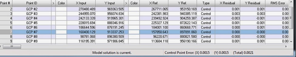
Figure 3a shows the reference image sierra_leone_east1991grf.img (right) and the distorted input image sierra_leone_east1991.img (left) as they appear in the Multipoint Correction interface prior to geometric correction. Figure 3b show the total control point (RMS) error.

l)              Once the RMS value is at the appropriate level, click Display Resample Image button at the top of the Multipoint Correction interface.

m)        Name the output file sl_east_gcc.img.

n)         Change the Resample Method to Bilinear Interpolation and click OK to run the model.

o)         Click Dismiss when the model is finished running. DO NOT SAVE CURRENT GEOMETRIC MODEL.

 

Q6 What type of map coordinate system is the reference image in?

UTM (Zone 29) projected coordinate system.

Q7What is the minimum GCPs you need to collect to perform a 3rd order polynomial transformation?

10 is the minimum number of GCPs needed to perform a 3^rd-order polynomial transformation.

Q8 Why is the Multipoint Geometric Correction interface reporting that model has no solution even though you have collected up to 9 points but for part 1 above, once you had 3 points your model reported that “Model solution is current”?

Since the transformation is a 3^rd order polynomial, more GCPs need to be placed on the Sierra Leone images than the Chicago images which used a 1^st-order polynomial transformation in order to geometrically correct them.

Q9 How geometrically correct is your rectified image compared to the reference image you used?

Figure 4 a-c shows the rectified image overlaid on the reference image in Erdas at various swipe stages. The rectified image seems to fit nicely over the reference image; however, 4d shows that the southeast corner of sl_east_gcc.img is not a perfect fit in this particular location.

Q10 Why was a bilinear interpolation resampling selected above instead of nearest neighbor as executed in part 1?

Bilinear interpolation (BLI) was used as a resampling method because it will produce a smoother image than nearest-neighbor (NN) will. Also, because BLI uses a weighted average of the four nearest pixel values, it is more accurate than NN. However, the accuracy gained in using BLI is done so with greater computational expense compared to NN.

Figure 4

a)                                                                                      

 

b)

 

c)                                                                                           

 

d)

Figure 4 a-c shows the rectified image sl_east_gcc.img in various Swipe-Function stages as it overlays the reference image sierra_leone_east1991grf.img. Figure 4d shows the SE corner of the two images, illustrating how this particular corner was poorly rectified.