Lab 8: Spectral Signature Analysis

Goal:

The purpose of this lab is to gain experience in the interpretation of spectral signatures of various earth features and surfaces. Twelve spectral signatures (SS) will be collected from the Eau Claire region using the polygon function in Erdas Imagine 2013. Once this is done the SS will be graphed the Signature Editor tool in Erdas.

Methods:

The polygon tool in Erdas imagine was used to spectrally isolate twelve regions around the Chippewa Valley, shown as a whole in figure 1, as such:

1)      Standing Water: This SS was taken from Lake Wissota near Eau Claire (EC), Wisconsin. Care was taken to retrieve the SS from the center of the lake to ensure the water was still.

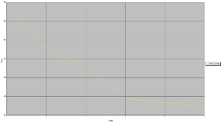
2)      Moving Water: This SS was retrieved from a known high-velocity region of the Chippewa River; just west of the UWEC campus.

3)      Vegetation: SS for forest vegetation was taken near Knapp, Wisconsin, where numerous forested areas are known to exist.

4)      Riparian Vegetation: SS for riparian vegetation was taken along the Chippewa River, just north of Lake Wissota.

5)      Crops: SS for cropland was taken just west of the area where the Lake WIssota standing water SS was taken.

6)      Urban Grass: The SS for this surface was taken from a golf-course just to the west of Altoona, WI.

7)      Dry Soil (uncultivated): This SS was taken from an open, uncultivated field near Knapp, WI.

8)      Moist Soil: SS for moist soil was taken near Knapp, WI as well. However, the location of this particular field was in a valley, where moisture retention would likely be higher due to runoff and shade.

9)      Rock: The SS signature for exposed rock was taken near Big Falls, WI, where massive units of bare bedrock line the Eau Claire River.

10)   Asphalt Highway: The SS for this location was taken on a paved road in the city of EC.

11)  Airport Runway: This SS was taken at the regional airport in Menomonie, WI.

12)  Concrete Surface (parking lot): A SS was taken of the concrete Sam’s Club parking lot in the city of EC.

Figures 2 through 13 show the graphical representations of the SS that were collected above. Also, table 1 shows the high and low bands for each SS obtained above.

Table 1.

Uncultivated*

 Figure 1

Overview of the Chippewa Valley region where SS were taken for this lab.

Analysis:

Water (figures 2 and 3):

Similar spectral signatures (SS), in terms of graph distribution and/or overall reflectance, a mostly seen in features that are comprised of similar materials. For instance, although standing and moving water, the SS of which are illustrated respectively in figures 2 and 3, vary in terms of overall reflectance, their minimum/maximum values on the graphs in figures 1 and 2 are located at similar bandwidths; in this case bands 4/6 (min.) and 1 (max.). One reason for the similarities in these SSs as represented on the graphs is that they both represent water, which generally reflects most EME in the visible spectrum (bands 1-3, but especially 2). In contrast, EME in other bands is absorbed by water, resulting in less reflectance and, thus, lower overall reflectance in these bands.

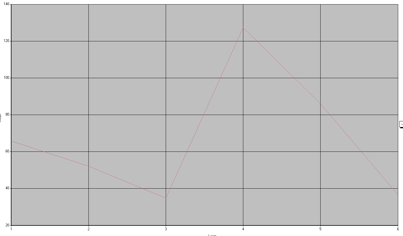
Vegetation (figures 4, 5, 6, and 7):

  Similarly, the SSs represented by various vegetation should exhibit graphic similarities to one another as well. This is exactly the case for SS collected from forest, riparian, and crop vegetation, whose graphs are represented in figures 4, 5, and 6, respectively. In fact, the SS values, in addition to the behavior of their graphs, for both forest and riparian vegetation were nearly identical. This could have arisen from the fact that the data for both features was collected in similar locations. For instance, one would expect that riparian vegetation would have plenty of water and would be generally healthy.

  Since SS data for the forest vegetation was collected near Knapp, WI, a hilly area with many valleys, it would not be surprising that data taken here would exhibit similar qualities. This is so because moisture would be less likely to evaporate from valleys than from more open areas. So, assuming a positive correlation exists between a plant’s access to water and its overall health, it would not be surprising that healthy vegetation, even from two separate locations, would have similar SSs; both in terms of graph values and behavior.

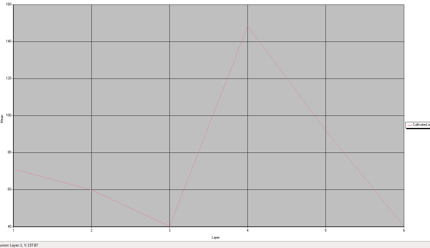
  Crop vegetation, figure5, had a higher maximum mean SS than either riparian or forest vegetation, about 150 versus about 130; all in NIR band 4. This overall greater reflectance exhibited by the SS of cropland compared to the SSs exhibited by riparian and forest vegetation could be due to the fact that light hitting cropland will be diffused less so than trees that inhabit forest and riparian environments. Also, cropland would likely be healthier overall because human intervention such as fertilization, regulated watering, and genetic modifications that are implemented by seed companies in order to ensure hardier crops.

 However, one type of vegetation did differ from the three mentioned above: urban grass. SS data for this feature was taken from a golf course near Altoona, WI (figure 7). While most of the graphic information for the SS of this feature was similar to that of riparian, forest, and crop vegetation, the SS of urban grass exhibited higher reflectance in both the band 1 and band 5, likely due to the fact that golf course grass would contain a lot more water compared to the types of vegetation mentioned previously.

Uncultivated Soil (figures 8 and 9):

While the spectral signature of both moist and dry soil exhibited a similar pattern on each graph, figure 8 shows that the overall reflectance of dry soil was the greater across all bands when compared to the reflectance of moist soil (figure 9). This is because the moisture contained within the soil will absorb EME more readily than dry soil.

  One note on these surfaces, however, is that the actual moisture content of the soil was merely speculated. For instance, the data for moist soil was collected from an uncultivated field in a valley. The assumption being that moisture content of soil would be higher in a valley setting due to factors such as less wind, less direct sun, and more forest vegetation, as well as topography that may channel runoff to such a location. In contrast, the data for dry soil was collected from a flat area with few trees to offer protection from sun and wind that could dry out the soil. However, the actual soil content of this location is unknown.

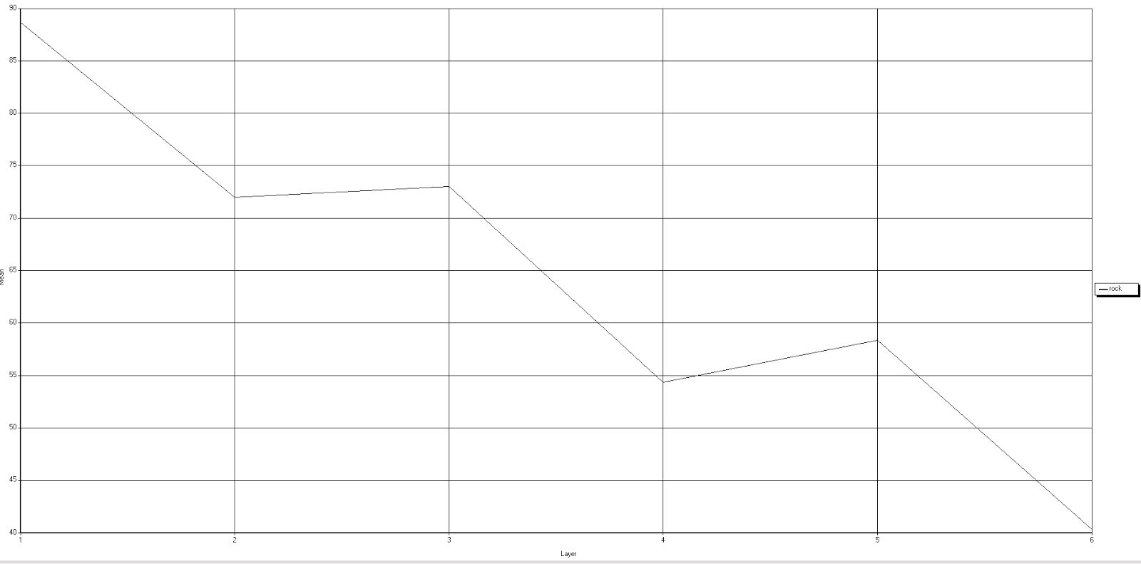
Rock (figure 10):

  Of all the hard-surface SSs listed in this lab (i.e. asphalt, rock, and concrete), bare rock (figure 10) had the least reflectance and graphical representation of the data that was least like the other three. One reason for this is that the location of this data was on the Eau Claire River (ECR) near Big Falls in Wisconsin. The bare rock in this area is likely too small for the spatial resolution of the image (30m). Because of this the spectral data of the water flowing through this location was likely averaged into the overall brightness value of the area. Other factors that may contribute to the high absorption of EME in this area is that the rocks themselves are dark in color and shadows on them may contribute to higher absorbance of EME in this area.

Asphalt, and Concrete (figures 11,  12, and 13):

  The SS of asphalt on a road surface (figure 11) had the least amount of reflectance compared to those of a runway and a concrete parking lot. One reason for this is that dark colored asphalt will absorb more EME due to its dark color compared to lighter colored asphalt or concrete.

  Figures 12 and 13 (runway and concrete, respectively) have very similar spectral signatures in terms of the way their graphs are patterned; at least compared to the SS of the asphalt surface shown in figure 11. This is likely due to the fact that these surfaces are much lighter, in terms of color, compared to asphalt and thus reflect more EME. However, the overall reflectance of the concrete Sam’s Club parking lot is greater than that of the runway.

  One reason for the similarities between the SS of the surface features at Sam’s Club and the Menomonie airport runway may be that they are both constructed of similar materials: concrete. However, differences in the spectral signatures Sam’s Club and the runway may be due to the fact that as airplanes land they leave skid marks from their rubber tires. Because of this, the overall reflectance between these two surfaces is different. With the more lightly colored parking lot reflecting more EME than the runway.

Figure 2

 

Spectral signature of water in Lake Wissota.

 Figure 3

Spectral signature of moving water (Chippewa River).

 Figure 4

Spectral signature of forest vegetation near Knapp, Wi.

 Figure 5

Spectral signature of riparian vegetation. Along Chippewa River, north of Lake Wissota.

 Figure 6

 

Spectral signature of cropland (cultivated). Near Eau Claire, Wi.

 Figure 7

 

Spectral signature of urban grass. Golf course near Altoona, Wi.

 Figure 8

Spectral signature of dry, uncultivated, open field near Knapp, Wi.

 Figure 9

Spectral signature of moist soil in. Uncultivated field in a valley near Knapp, Wi.

 Figure 10

 Spectral signature of rock at Big Falls along the Eau Claire River.

 Figure 11

 

Spectral signature of asphalt on an Eau Claire road.

 Figure 12

Spectral signature of an airport runway (Menomonie, Wi).

 Figure 13

Spectral signature of a concrete parking lot (Walmart, Eau Claire, Wi).

Lab 7: Photogrammetry and Orthorectification

                         

Goal:

  This lab was an introduction to photogrammetry skills that can aid in the analysis of aerial photographs and satellite images. Techniques used to complete this lab were calculating scales from various aerial photographs, calculating relief displacement, and digitizing features within the Erdas viewer in order to calculate their areas. Also, Lecia Photogrammetric Suite was used in order to create a planimetrically-true orhtoimage.

Part 1: Scales, Measurement, and Relief Displacement:

Section 1: Calculating Scale of Nearly Vertical Aerial Photographs:

The following equation was used to calculate the scale of Eau Claire_West-se.jpg, shown in figure 1.

 

S = [pd/gd]   

Where:

S = Scale

Pd = Photo Distance = 3”

Gd = Ground Distance= 8822.47’ = 105869.64”                       [1]

Using equation 1 and multiplying the denominator by 3, the calculations should be as follows:

 

     9.44564E-6 ≈ 1/105869.64  

So the scale for this map after rounding is 1:110000.

Next, focal length and altitude was used to calculate the scale of ec_east-sw.img:

                     

                         S = [f/(H-h)]                                                                                                 

                         Where:

                         f= focal length of lens = 152mm 5.9843”

                         H= altitude above sea level = 20000’ = 240000”

                          h= elevation of terrain=796’ = 9552”                                 [2]

                   Using equation 2 and multiplying the denominator by 5.9843, the calculation will

                   be as follows:

                    4.33937E-6 ≈ 1/230448

          So the scale of this map after rounding is 1: 230000.

 

Figure 1

Figure 1 shows an example of how Eau Claire_West-se.jpg should look.

 

 Section 2: Measurement of Areas of Features on Aerial Photographs:

The lagoon in ec_west-se.img (figure 2; marked with an ‘x’) was digitized and measured using the polygon tool in Erdas Imagine to calculate its area. Following is a list of the results.

Hectares ≈37.99 hectares

Acres ≈ 93.87 acres

Meters ≈ 379888m²

Miles ≈ 0.1467 miles²

 

Figure 2

Figure 2 shows the lagoon that is to be measured in section 2 of this lab.

 

Section 3: Calculating Relief Displacement From Object Height:

 

The relief displacement of the smokestack in relief_displacement_1.jpg  was calculated using the following equation (map scale is 1: 3209):
 

d=[hr/H]

 
Where:

d= relief displacement ≈ 0.2457

h= height of object (real world) = (0.375”)x(3209”)=1203.375”

r= radial distance from the top of the displaced object from principal point (photo)=9.75”

H= height of camera above local datum = 47760”                                                                               [3]

Figure 3 shows what Relief displacement_1.jpg should look like once it is opened.

Figure 3

Figure 3 shows relief_displacement_1.jpg. However, the calculations using equation three must be performed when the above file is displayed in an appropriate photo viewer and not in this figure.

 

Part 2: Stereoscopy:

In this section of the lab, a digital elevation map (DEM) was used to create an anaglyph. This was done in order to show elevation changes in the Eau Claire area. The results had a stair-stepped appearance where elevation change was abrupt. This effect likely had to do with the differences in spatial resolution between the two images (i.e. 10m on the DEM and 1m on the city image it was merged with).

Also, a second image was created where the only change was made to the vertical exaggeration to see how this would affect the SS effect. When this was done the SS effect occurred in different locations on the second image as compared to the first.

Part 3: Orthorectification:

The goal of this section of the lab was to:

1)      Create a project using Erdas Imagine Lecia Photogrammetric Suite.

2)      Select a horizontal reference source.

3)      Collect ground control points (GCP) in the first image.

4)      Add a second image to the block-file.

5)      Collect GCPs in the second image.

6)      Perform automatic tie-point collection.

7)      Triangulate the images.

8)      Orthorectify the images

9)      View the orhtoimages.

10)  Save the block-file.

Methods:

1: Create a new project:

a)      Two images, spot_pan.img and xs_ortho.img, were used as the initial input images.

b)      A model was set up using Polynomial-based Pushbroom as its Geometric Model Category.

c)      The UTM (Zone 11, North) projection was used in the Block-Property set up, with Spheroid: Clarke 1886 and Datum: NAD27 (CONUS).

2: Add imagery to the block and define sensor model:

This section of the lab determines what the internal coordinate system will be. That is how the camera was oriented when it captured the image. Nothing was changed in this lab.

3: Collect GCPs (x, y, and z) of the first block file spot_pan.img:

a)      xs_ortho.img was the image that

b)      Measurement tool was Classic Point.

c)      A total of 11 GCPs (x and y) were spatially synchronized on the spot_pan.img and spot_panb.img.

d)      The DEM image palm_springs_dem.img was used to obtain z-coordinates for the orthorectified image. This was done to provide a z axis (elevation) on the final image.

 

4: Set type and usage: These were set to full and control, respectively. This concluded the collection process for spot_pan.img.

5: Add a 2^nd (spot_panb.img) image to the block (spot_panb.img) & collect its GCPs:

Collection of GCPs in this section was identical to those collected in the previous steps.

 

6: Automatic tie-point collection:

Tie-points will be collected in this section of the lab in order measure image coordinate system at overlapping regions of the spot_pan.img and spot_panb.imgs.

a)      General tie-point properties were set as follows: Images: All; Initial Type: Exterior/Header/GCP.

b)      Distribution: Intended Number of Points per Image was set at 40.

7: Triangulation:

Triangulation was performed using the following parameters:

a)      Iterations With Relaxation: 3.

b)      Image Coordinate Units for Report: Pixels.

c)      Type of Point: Same Weighted Value.

d)      x,y, and z: 15.00000.

e)      Simple Gross Error Check Using: 3 times of unit weight.

8: Ortho-resampling:

a)      DEM Source: palm_springs_dem.img

b)      Output Cell Sizes (x and y): 10.

c)      Resample Method: Bilinear Interpolation.

 

Output Images:

Shown below in figure 4a, the overall spatial overlap at the boundaries of the orthorectified images (orthospot_panb.img overlaying orthospot_pan.img) is accurate. However, when zooming in close some sections of the boundaries are not matched perfectly between the images. For instance, figure 4b shows the ‘Swipe’ view of panb overlaying pan at an extent of about 1:11000 in the Erdas viewer. Notice that at the boundary between the two images the river features do not match up.

  Since this effect does not occur throughout the image, it may have to do with the accuracy of individual reference points. For instance, if a reference point was slightly inaccurate on either input image or the DEM, then when resampling occurred that inaccuracy might be transferred to the output image(s) once Ortho-resampling was applied.

 

Figure 4

a)

b)

Figure 4a shows the two orthorectified images, orthospot_pan and orthospot_panb in the Erdas viewer; panb is overlaying pan in this case. Figure 4b details the square in 1a and shows some inaccuracy of the spatial overlap between the two images (circle).